The Value Of Material Things IIa
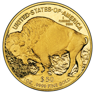
If a GP is 18-carat gold (see text), then this would weigh about as much as 1 1/2 of them. I think. Image by WikiImages from Pixabay
First, A Correction (and some expansion)
I wasn’t going to be talking about this stuff today. I’ve done almost half of the third “Strange Places” article, and that was my intended post of the week.
But….
When I calculated how much a Gold Dime would weigh last week, I uses diameter instead of radius. This has a big impact, as you will see:
What if a dime were made of gold?
There’s a purpose to this. For a start, a dime is roughly the size that I think of when I think GP. It For another, it’s a fairly ubiquitous coin size – not far away from the Australian 10-cent piece for example. And for a third, if I can say that a GP is the size of a dime, but the weight of × dimes, everyone will be able to relate to the numbers.
Weight (real dime) = 2.268g
Diameter = 17.91 mm = 1.791 cm
Radius = 1.791 / 2 = 0.8955 cm (that’s the step that I missed)
Thickness = 1.36 mm = 0.136 cm
Volume in cubic cm = pi × r^2 × ht
= 3.1416 × 0.8955 ^ 2 × 0.136 = 0.3426 cm^3.
Density of pure gold = 19.3 g / cm^3
so weight = 6.6127 g
= 2.91 regular dimes.
Three dimes would be a fraction heavy – about 2.8%.
Value, 24 ct = 6.6127 / 313.54573 × 20067 = $423.21 USD.
Value, 18 ct = $317.41.
Value, 15 ct = $264.51.
But 15-ct gold would also reduce the weight – not all the way to 62.5%, because whatever impurities there are have to weigh something, but that’s a start. 6.6127 × 62.5% = 4.133 g = 1.823 regular dimes.
My instincts throughout the remainder of last week’s post were that the value of $1058.03 was too high, by a factor of around 10, and 1/2 cubed is 1/8th. So my instincts were right, but misinterpreted.
Let’s scale that up a little: Ten gp = 18.23 g = almost exactly 8 regular dimes. With (at 15-ct), 37.5% impurities – even if they weigh only about 20% as much as gold – that would add 8 × 37.5% × 20% × 1.823 / 2.268 = 0.48 additional dimes, 1.0938 g.
That’s the weight of a paperclip, or a 1$ note.
But, given that value is no longer the crisis that it appeared to be last week, let’s go back to 18-ct gold and see what we get.
Value, 18 ct = $317.41.
Weight, 18 ct = 75 × 4.133 g / 62.5 = 4.9596 g
= 2.1868 standard dimes.
10 standard dimes = 4.573 gold dimes..
5 gold dimes = 10.933 regular dimes.
Now we’re getting somewhere!
Good Meal Test
So let’s see where we’re at with the Good Meal Test.
A really good meal for 1 will cost about 1 gp (I call this the “Good Meal” standard). It will also cost $50-100 modern Australian dollars at the extreme, but $18-$30 is more reasonable, and that’s what I’ve been using as my yardstick. If I convert those numbers into US dollars at last week’s exchange rate, I get:
$100 AUD = $63.76 USD
$50 AUD = $31.86 USD
$30.AUD = $19.13 USD
$18 AUD = $11.48 USD
So US $19-32 would be a reasonable first estimate for the value of a GP, and more probably at the lower end of that range. $20 or $25 would seem about right.
The common meal standard
.This works on a 1/10th gp conversion. A mid-quality bog-standard common meal, consumed by thousands of people a day both here and everywhere else, will cost $10-$20 AUD, and closer to the top end of that range.
Apply the same exchange rate:
$10 AUD = $6.38 USD
$20 AUD = $12.76 USD
So, the equivalence is suggesting that 1/10th of a gp is around US $9-12, and therefore a GP is going to be worth somewhere close to USD $105.
That’s a big difference, but it’s not as extreme as the factor-of-ten that we got last time. Let’s try to reconcile the two values using the math tricks from last week:
Mathematical Trickery
Average of $105 and $20 = $62.50
Average of $105 and $25 = $65
$105 × $20 = 2100, square root = $45.80.
$105 × $25 = 2625, square root = $51.20.
Average of $62.50 and $65 = $63.75
Average of $45.80 and $51.20 = $48.50
Average of $63.75 and $48.50 = $56.13
$62.50 × $65 = 4062.5, square root is $63.74.
$45.80 × $51.20 = 2344.96, square root is $48.42
$63.75 × $48.50 = 3091.875, square root is $55.60
We seem to be honing in on a value of around $55.50. We have much bigger margins of error than 50 cents, so lose that and we get a rough conversion rate of
I GP = $55 USD.
The values that we got to last week were $23.34, $40.59, and $18.77. This is 2-3 times two of those values, and about 20% higher than the third.
A lot hinges on how many gp you would pay for a really good meal, in-game. If 1-2 gp, the $55 value is going to be the sort of number you should pick. If 3-4, I would set it to about $25.
From last week’s article:
Once you have that number, you can take a gem result – be it 1 gp, 10 gp, 50gp, 500gp, 5000gp, or 50,000 – and get the USD equivalent. Once you have that, and the information contained in this post and last week’s, and you can directly determine the weight and dimensions of the gem.
Special gems are easily handled simply by multiplying the base value of a 1ct gem with those special characteristics by an appropriate factor – times 1.5? Times 10? Times 100? – it’s up to you.
What’s more, if you do a little prep work and save the results, you can define a standard gem – in your game world – and up-scale or downscale it as needed.
Value / base 1-ct value will always give you the square of the number of carats. So if the dice say a 10,000 gp gem, you can simply divide by your base value, take the square root, and you have the number of carats.
New Thoughts On Depreciation & Appreciation
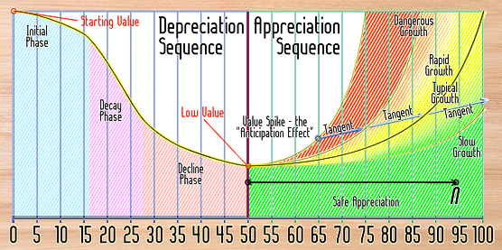
The diagram above is a little hard to read because I had to fit it into Campaign Mastery’s column size. I was going to provide a link to download a larger version, but then I realized that I could simply show both halves – slightly larger than full sized!
So lot’s do that, then.
Depreciation Sequence
It might nor seem it, but this is actually a far simplified model of the process.
Depreciation isn’t really a constant change, despite all attempts to treat it that way by accountants. There are three phases –
- an initial phase in which the real value doesn’t decline by much, which I have named the “initial phase”;
- a middle phase in which real value is lost rapidly; which I have named the “decay phase”; and
- a period in which depreciation slows and almost stops.
Overall, we have a total of 50 years. The decay phase is 10-20 years in the middle, probably closer to the 20 end of the scale. That leaves just over 30 years to account for.
The decline phase is going to be about 1½ times the length of the initial phase, so dividing 30-plus-a-couple by 2½ gets us the length of the initial phase – 12-13 years. Yes, I’ve shown it as too wide and the decay phase as too short. Never mind that.
If we call it 12 years, that uses 20 years exactly for the decay phase, and leaves 18 years for the decline phase. But, let’s simplify further and call the phases 10, 20, and 20 years in length.
A more technical approach
If you wanted something less arbitrary, the initial phase persists until the object has lost 20% of it’s value, or 15 years have passed – whichever comes first.
The Initial Phase
In the initial phase, decline in real value is much less than the accountants would have us believe. They want a flat rate that erodes a certain amount every year, in other words a formula that reads:
V2 = V1 × r ^ (T / I), where
V2 = the depreciated value,
V1 = the starting value,
T = the age of the object,
I = the interval of measurement, and
r is the depreciation rate over a span of the interval of measurement.This is what I’ve been trying to use, and it’s a pain because it’s so sensitive to both age and to the depreciation rate.
Whatever your base depreciation rate is, in the initial phase it will be a lot less. Generally:
R(i) = [ 2 + R(b) ] / 3
will be about right.
Let’s compare that against a 10% depreciation rate, commonly used for motor vehicles and a 20% rate used for more perishable objects like furniture:
We’ll start with an object valued at a nice round $1000.
R1 = 100-10% = 0.9.
R2 = 100-20% = 0.8
R3 = (2+0.9)/3 = 0.9667.
1 year @ R1: v = 1000 × 0.9^1 = 900.
2 years @ R1: v = 1000 × 0.9^2 = 810.
3 years @ R1: v = 1000 × 0.9^3 = 729.
4 years @ R1: v = 1000 × 0.9^4 = 656.10.
5 years @ R1: v = 1000 × 0.9^5 = 590.49.
6 years @ R1: v = 1000 × 0.9^6 = 531.44.
7 years @ R1: v = 1000 × 0.9^7 = 478.30.
8 years @ R1: v = 1000 × 0.9^8 = 430.47.
9 years @ R1: v = 1000 × 0.9^9 = 387.42.
10 years @ R1: v = 1000 × 0.9^10 = 348.68.
1 year @ R2: v = 1000 × 0.8^1 = 800.
2 years @ R2: v = 1000 × 0.8^2 = 640.
3 years @ R2: v = 1000 × 0.8^3 = 729.
4 years @ R2: v = 1000 × 0.8^4 = 512.
5 years @ R2: v = 1000 × 0.8^5 = 409.60.
6 years @ R2: v = 1000 × 0.8^6 = 327.68.
7 years @ R2: v = 1000 × 0.8^7 = 262.14.
8 years @ R2: v = 1000 × 0.8^8 = 209.72.
9 years @ R2: v = 1000 × 0.8^9 = 167.77.
10 years @ R2: v = 1000 × 0.8^10 = 134.22.
.
1 year @ R3: v = 1000 × 0.9667^1 = 866.70.
2 years @ R3: v = 1000 × 0.9667^2 = 934.51.
3 years @ R3: v = 1000 × 0.9667^3 = 903.39.
4 years @ R3: v = 1000 × 0.9667^4 = 873.31.
5 years @ R3: v = 1000 × 0.9667^5 = 844.23.
6 years @ R3: v = 1000 × 0.9667^6 = 816.11.
7 years @ R3: v = 1000 × 0.9667^7 = 788.94.
8 years @ R3: v = 1000 × 0.9667^8 = 762.66.
9 years @ R3: v = 1000 × 0.9667^9 = 737.27.
10 years @ R3: v = 1000 × 0.9667^10 = 712.72.
.
If these rates persisted for the full 50 years:
50 years @ R1 = $5.15.
50 years @ R2 = $0.01 (0.015 if you prefer).
50 years @ R3 = $183.90.
Even a single percentage point can make a large difference as it compounds over the years.
I don’t know how others treat their possessions, but a year after I buy mine, unless something extraordinary has happened, they are still in almost new condition. No way have they lost a tenth of their value, let alone a 20th.
There are exceptions – computers, electronics, and high-tech of other sorts, and anything that sees excessive wear-and-tear or significant daily use, like mattresses.
The Decay Phase
This is where the full rate kicks in, plus a bit more to make up for the slower rates at beginning and end.
Essentially, at the end of the Decay Phase (should it persist for the full 20 years), the object will have lost sufficient value that it will be where the accountant’s formula would have predicted.
Technically, that means working out what that value would be and then reverse engineering to get the 20-year rate:
V1 = V × r1 ^ (20+ITP)
V2 = V × r2 ^ (ITP)
V2 = (V2 – V1) × r3 ^ 20, so
V2 / (V2 – V1) = r3 ^ 20
log [ V2 / (V2 – V1) ] = 20 × log [r3], i.e.
log [r3] = 1/20 × log [ V2 / (V2 – V1) ]
eg: r1= 10%, V = 1000, r2=3.33%, ITP = 12 years:
V1 = 1000 × 0.9 ^ (20+12) = 34.34
V2 = 1000 × 0.9667 ^ (12) = 666.04
log [r3] = 1/20 × log [ 666.04 / (666.04 – 34.34) ] = 0.0011495;
r3 = 1.00265 — which makes no sense, the rate has to be <1.
Back to First principles:
666.04 -> 34.34 in one step = x0.05156.
in two steps: square root of 0.05156 = x0.22707.
log Y =log [ 0.05156 ] ^ 1/2 = -0.64384;
Y = 0.22707. Technique confirmed.
therefore in 20 steps: 20th root of 0.05156;
log [0.05156] / 20 = -0.064384; Y = 0.8622.
Check: 666.04 × 0.8622 ^ 20 = 34.33.
So the depreciation rate in the decay phase is 13.78% – that’s what we need to get the depreciation back ‘on track’..
A rough shortcut
0.79228 in one step = × (0.79228 / 666.04) = × 0.00119
in two steps: square root of 0.000119 = × 0.0345
therefore in 20 steps: 20th root of 0.00119;
log [0.00119] / 20 = –0.1462226; Y = 0.71413
So the depreciation rate in the decay phase is 28.587% – that’s what we need to get the depreciation back ‘on track’..
Using our shortcut: 20 × 1.4 = 28%.
20 years @ 28.58%, start $666.04: $0.79
20 years @ 28%, start $666.04: $0.93.
14 cents. But that’s close enough for me.
A premature end
The decline phase can finish early – basically, if the value of the object drops to less than 5% of it’s original value, or less than $1, whichever comes first, plus one more year.
V2 = 5% of 1000 = $50
Our 10% drop carried us to $34.33, which is below $50. The rate was × 0.8622.
So the 19th year, we had a value of 34.33 / 0.8622 = $39.82.
The 18th year, we had a value of 39.82 / 0.8622 = $46.18.
The 17th year, we had a value of $53.56.
In this case, the decay phase ends after 18 years, adding 2 to the length of the decline phase.
Our 20% drop gave a value of $0.93, at a decline of – using the shortcut – 28%.
Year 19: 0.93 / 0.72 = 1.29
Year 18: 1.29 / 0.72 = 1.79 (okay, that’s enough of showing the working)
Year 17: 2.49
Year 16: 3.46
Year 15: 4.81
Year 14: 6.68
Year 13: 9.27
Year 12: 12.88
Year 11: 17.89
Year 10: 24.84
Year 9: 34.50
Year 8: 47.92
Year 7: 66.55
So the Decay phase stops after a brutal 8-year run and a value of $47.92. And the decline phase gets an extra 12 years tacked on.
Still more technical nuance to ignore
If you want to get technical, the rate itself in the Decay Phase starts off at the initial rate and changes over time to get to the correct value. But that’s too messy. The product of a series of products – I did some of that stuff back when I was doing higher calculus. No thanks.
The Decline Phase
Fortunately, the decay phase is time-limited. The decline phase then takes over, in which the devaluation effect starts at what was initially specified for the overall rate and moderates back to the initial value.
Again, that’s too much like work. So let’s use another shortcut:
[R1 × (T-1) + R2 ] / T
Let’s say it’s 22 years, the 10% example.
T=22, R1 = 0.9667, R2 = 0.8622.
21 × 0.9667 + 0.8622 = 21.1629
21.1629 / 22 = 0.96195.
A more realistic calculation would be (2/3 × R1) + (1/3 × R2).
(2/3 × 0.9667) + (1/3 × 0.8622) =
0.6444467 + 0.2874 = 0.9318.
Since this is significantly different from the simpler calculation, it is the recommended technique.
The Appreciation Sequence
So, one way or the other, you’ve gotten to the bottom of the curve. The object (assuming it has survived) will never be worth so little again.
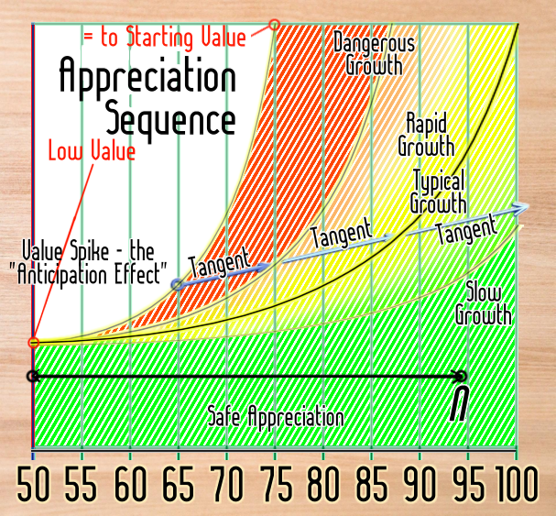
Although it looks more complicated, this is actually a much simpler side to things. Of course, it’s possible to complicate things, but if you don’t have to, why bother?
The value of the object starts at the minimum determined in the depreciation stage and starts to grow – just a little each year. I’ve been using intervals of 20 years, but this diagram is marked in 5-year intervals.
At first, there’s hardly any change. It will be barely noticeable at the 60-year mark. But significant differentiation can take place at the 15-year mark.
This graph illustrates four different rates of appreciation. I’ll get to them in a moment.
A critical value is N. This is the number of time-intervals at which all the losses due to depreciation have been reversed, wiped out by the increasing value.
As soon as you cross that line, you can set depreciation to zero and simply subtract 50-n from your object age. From that point on, it will only increase in value – all other effects notwithstanding, of course.
N is the date at which you can ignore depreciation entirely.
Clearly, each of the growth rates will reach that point at a different date.
It’s also not uncommon for an appreciation rate to change after that landmark value, but that’s an unnecessary complication.
Value Spikes and the Tangent
If you expect an item to rise in value over the next X years, there is a temptation to factor that growth into the price you’re willing to pay today.
This causes the “value” to spike. It may even appear to be following the dangerous growth curve!
Once this initial spike is registered, however, the value increase flattens into a straight line – the tangent – until it reaches the correct value-growth curve for this item, at which point, “normal” growth will resume.
This tangent can be (usually is) upwards; it can be flat; it can even be downwards, though that only happens in more extreme spikes.
Spike severity is measured in the number of years of anticipated growth are incorporated into the value paid / demanded for the item.
If the example above were to the “typical Growth” curve, for example, at around the 82-year mark, the value would match the purchase price shown at age 65 – so that’s 82-65 = 17 years of increase.
- 1-5 years of increase: a minor ‘bump’ in the price. Almost negligible. Expect a rising tangent.
- 6-10 years of increase: officially qualifies as a ‘speculative investment’, though a fairly conservative one. Expect a flat Tangent, or one that is slowly rising. The line shown above would be about the most extreme.
- 11-20 years of increase: speculative, and not entirely safe. The tangent will be flat, rising very slightly, or even falling slightly.
- 21+ years if increase: highly speculative and extremely risky. Tangents are almost certainly downwards, and between 30° and 45° in slope (50 years × 100% graph)..That generally means that in 10-15 years, the tangent will intersect the true value line.
Slow Growth
Slow growth is safe, steady, and stately. Everything eventually achieves this growth rate.
Precious Metals and Gemstones are usually slow growers. But so is real estate. “Safe As Houses”, anyone?
Typical Growth
Objects that were once valueless or mundane, if nicely decorated, tend to follow the typical growth curve, which takes about 50 years to erase the impact of depreciation. Adjusted for inflation, a 100-year-old vase will be worth roughly what it was worth when new.
That adjustment for inflation is a killer, though. Shrinkage in the value of the dollar can be a 30- or 40-fold change in a century. So a $30 object can be priced at $750 – and still not have reached its initial value ($900 equivalent).
Objects of especial merit or value can appreciate still faster – an N of less than 50, in other words.
Up to ten years early (an N of 40) is tolerable, and signals an object of active interest to collectors. Anything faster and you start taking risks, albeit small ones at first.
Typical Growth is not without its risks, largely in the form of collateral damage to some more extreme fall in value. Such effects are generally minor and temporary; in the long run, they are little more than a rounding error. Value growth may be delayed but will make it up in the long-term.
Dangerous Growth
The dangerous growth line is set to an N of 25 and this marks a threshold to be crossed only at your peril. Anything faster than this is almost certain to suffer a value collapse – possibly even within the 50-year appreciation span showing. The growth in value is (generally) unsustainable.
It is so fast that it will attract counterfeiters and thieves and the costs involved (provenience in the first case, protective security in the second) directly detract from the value. Not having an object on display because it’s too dangerous also subtracts from its value, both in a slower appreciation rate and losses in social desirability.
The red zone a roller-coaster – and it can plunge values to close to zero, no matter what they started at – all corrections always over-correct. Look at what happened to the Dutch Tulip market.
Over $1000 in the currency of the time (or it’s equivalent) for a single bulb? This way lies lunacy! I’m sure investors who were caught in the dot-com bubble-burst can empathize.
Everything that I’ve seen suggests that most cryptocurrencies, like Bitcoin, are following a similar trend path. Several of them have crashed in value and even ceased to exist over the last few years.
Artworks and Exceptions
But there’s an exception to this rule – artistic merit tends to be conserved. While a few artists have lost value over the years, the worst that tends to happen is that they stabilize onto a slow or even very slow growth curve.
Of course, such a curve might not keep up with inflation, causing a drop in real value. But even that is rare.
An exception to the exception comes in the form of signatures – these gain their value through the name recognition accorded the (former?) owner of the signature, and if that fame diminishes, so will the value – perhaps precipitously.
Practical Matters
So, set the rate according to the age that you care about, determine the N accordingly, and simply start your appreciation from Base Value at year / interval N+1. You have all the tools you need.
Wow, that sure looks more like a typical post than I was expecting! Hope it’s worthwhile…

Discover more from Campaign Mastery
Subscribe to get the latest posts sent to your email.
Comments Off on The Value Of Material Things IIa


