All Over Bar The Shouting: Fantasy Tavern Generator Pt 6
- The Palomino and Fox (and other establishments)
- The Spotted Parrot (and other establishments)
- The Robber’s End (and other establishments)
- Going down to the pub: Mike’s Fantasy Tavern Generator Pt 4
- Draw Another Pint: Mike’s Fantasy Tavern Generator Pt 5
- All Over Bar The Shouting: Fantasy Tavern Generator Pt 6
Image provided by FreeImages.com/Benjamin Flux
Part one of this series used six tables to define the physical properties of a tavern (no guest accommodations) or inn (with guest accommodations), plus – because the modifiers needed were at hand – the meals provided by the kitchens.
Part two used another six tables to determine everything that directly contributed to the ambience of the establishment, from the personality of the owner through to the decorations on the walls. In this final part of the generator, we’ll deal with the bartender’s family and process the worksheets that bring the whole tavern or inn together, ready for use.
Part three used another five tables and subtables and one worksheet to populate the extended-family-in-residence and establish what entertainments the tavern provides to keep the punters happy. That was supposed to be the final part (aside from a behind-the-curtain techniques discussion to be written down the track), but the examples grew uncontainably large, so the decision was made to separate the worksheets from the final set of rolls.
Part four contained the first worksheet, and provided detailed instructions for use (together with some tips and tricks for getting exactly the result you want from the generator.
Part five contained tables 17a through 17h and 18a through 18d – everything needed to generate the second level of the tavern or inn, which is usually where the owners reside, and where there will be guest accommodations if the tavern is also an inn. But there wasn’t room for the examples.
Which brings me to this penultimate part in the series – Worksheets 19a through 19c, Tables 18f through 18j, and Worksheets 20a through 20i, which detail the remaining levels and the tavern patronage.
Still missing – squeezed out to make room for extra tables – is the completion of the examples, yielding three finished taverns for GMs to use in their own campaigns. And I have one additional “behind the scenes” article detailing many of the tricks and techniques used to create these tables, so that other GMs can use them.
I have to apologize for the lateness of this article, on two grounds.
First, it took a lot longer to write than expected – the length shows that I wasn’t dilly-dallying but it still took a long time. There were a couple of dead ends that I chased myself down; in the end, I generated more pages in hand-written notes for this one part of the series than for the entire rest-of-series put together.
Secondly, this should have posted yesterday, or – if it wasn’t going to be ready – reshuffled the publishing schedule to put up a filler article. I’ve done that before, and consider that to be a lesser evil than missing deadline. The problem is that this was so close to being finished that – while I knew it would be a tight squeeze – I was certain that it would be finished in time, give-or-take an hour or so.
I didn’t count on my brain frying late in the day – with about six hours work to go. I struggled on for several more hours at a diminishing fraction of my normal productivity, but by the end of my endurance I was still about three hours short of completion. Hence the delay – I not only had to do that three hours of work, but fix a mess of mistakes made while I was struggling.
So, Mea Culpa – I missed the deadline, but I got here in the end.

Tavern Generator (cont): Worksheets 19a-19c: Upper Floor Calculations Worksheets
As usual, we pick up the process right where we left off; the basic principles and general technique remain the same. Note that it is impossible to use this content without having completed the earlier parts of the process.
Table 19a: Second Floor Calculations Worksheet
In the process of working out what you were doing for the first residential level, you also made all the decisions necessary for all the other residential levels, so this worksheet is much simpler (and resembles Table 17h). To further simplify it, a cheat has been employed that uses any leftover space for storage – probably for linen, cleaning products and tools, and so on.
We start by allowing for a cheat that may have been specified earlier: the substitution of a “suite” for any family accommodations. If this option hasn’t been employed, any family accommodations on the first floor have to be replaced with additional guest rooms on subsequent floors. After calculating the number of relative spaces to be filled, we divide the result by the relative size of the guest rooms (and round down) to determine how many will fit, and note the result as (m). To this, we add the number of guest rooms located on the first floor.
With this total as a guide, we set the number of guest rooms to be located on this floor. You have many options here – the number can be greater than the guideline, indicating that this level of the inn is larger than the first floor, or smaller – refer to the sidebar that follows the table for some of the many options available to the designer.
I would also pay special attention to the amount of storage space from the first floor and how close to the next value up the rounding was in the division above – “2.9” will round down to 9, but if there was a lot of storage space on the first floor, you could allow a little less space for that purpose on this level by trimming the storage space.
Once you have determined how much space is consumed by guest accommodations (including connecting corridors), we make the usual allowances for stairs up (which there may not be, if this is the upper level of the inn), stairs down (which there have to be), any other spaces that have been designated as appearing on this level, and then determine the subtotal of allocated spaces. Subtracting this amount from the total indicates how much space is used for storage, since that’s the only purpose we haven’t set aside room for.
While you could continue down the worksheet at this point, while the particulars are all fresh in mind, I would calculate the actual sizes and adjust them, as usual, in the spaces on the right-hand trio of columns, before continuing.
After doing so, you move on to the third part of the table, in which you calculate the number of guests that can be accommodated on this level, and establish and maintain a running total of the total guest capacity. Once you have done so, you’re ready to progress to a third level, and even a fourth level, in exactly the same way.

| Instructions | Working | Calculated Areas [Relative Size x (l)] (from Part 5) |
Area Adjustments | Final Areas | |
|---|---|---|---|---|---|
| Size family accomm, 1st floor | |||||
| + relative size “other” 1st floor spaces = | + | = | |||
| – relative size suites on this floor = | – | = | |||
| / relative size guest quarters, round down = (m) | / | = | |||
| + # guest rooms, 1st floor = | + | = | |||
| # guest rooms, this floor (n) | = | ||||
| x rel size guest accommodations = | x | = | |||
| + stairs up = | + | = | |||
| + stairs down = | + | = | |||
| + other spaces (if any) = (o) | + | = | |||
| total spaces, 1st floor (guideline reference) | |||||
| total spaces, this floor | |||||
| – (o) = storage space this floor | – | = | |||
| total footprint, this floor | |||||
| total footprint, ground floor (for comparison) | |||||
| (n) | |||||
| – rooms occupied by extended family = | – | = | |||
| x #guests/room (range) = | x | = | |||
| + #guests in suites (if any) | + | ||||
| = #guests accommodated on this floor | = | ||||
| + #guests accommodated on previous floors | + | ||||
| = total guests accommodated | = | ||||
Sidebar: Possible layouts and relative level sizes
Below, I have illustrated half-a-dozen of the innumerable layout possibilities with reference to floor areas alone.
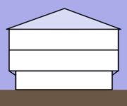
Figure 1
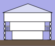
Figure 2
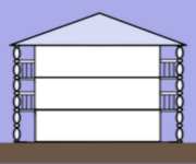
Figure 3
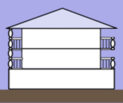
Figure 4
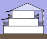
Figure 5
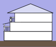
Figure 6
Figure 1 shows what is perhaps the most common and recognizable configuration. The ground floor is (slightly) smaller than the residential floors.
In Figure 2, the first floor is significantly larger than the ground floor, and has a balcony (not considered part of the footprint of the floor). The second floor is significantly larger again, requiring support from below. The balcony therefore forms a canopy over the surrounds of the ground floor. Two such buildings can be almost side-by-side, separated by mere feet, and there is still enough space to form an alleyway between them for foot traffic or access to an attached stables.
Figure 3 is another familiar layout. All three floors have the same footprint, but the above-ground floors have balconies (not considered part of those footprints). This is typical of the Western Saloon.
Figure 4 will also be familiar to most readers, especially those from Australia; it is that of the quintessential Outback Pub (or would be if it were not for the presence of a third level, which is uncommon). The two residential levels are smaller than the ground floor, permitting them to have balconies. Additional roof support is shown on the left-hand side, but might not be needed, as shown on the right.
Figure 5 is similar to the previous layout, but with each level progressively smaller, producing a more Mediterranean impression. Roof supports may or may not be needed, enabling awnings, as shown on the left. This does not work if roof support is needed, as shown on the right, but this arrangement – although it looks strange – ensures that each residential level is well-shaded, and hence may be found in hotter environments, or where construction materials of sufficient strength are not available.
There is absolutely nothing that states that buildings need to be arranged symmetrically, as Figure 6 illustrates. Each level is still smaller than the one below it, and it still has balconies and awnings, but what is obviously the back of the building presents a flat facade to whatever lies behind. There have also been occasions when what we consider the back in this illustration was in fact the front (and heavily reinforced against attack), with the balconies facing away from the source of danger; arrange many such structures next to each other without gaps, and you present a fortified “wall” to the world. However, this was more normal in cases of individual dwellings and not those providing public accommodations, because the strangers residing there would not be as readily trusted as known families. Nevertheless, string many such “buildings” of narrow width in a semi-detached row and you have something that would serve as an Inn.
Worksheet 19b: Third Floor Calculations
Instructions as per Second Floor.
| Instructions | Working | Calculated Areas [Relative Size x (l)] (from Part 5) |
Area Adjustments | Final Areas | |
|---|---|---|---|---|---|
| Size family accomm, 1st floor | |||||
| + relative size “other” 1st floor spaces = | + | = | |||
| – relative size suites on this floor = | – | = | |||
| / relative size guest quarters, round down = (m) | / | = | |||
| + # guest rooms, 1st floor = | + | = | |||
| # guest rooms, this floor (n) | = | ||||
| x rel size guest accommodations = | x | = | |||
| + stairs up = | + | = | |||
| + stairs down = | + | = | |||
| + other spaces (if any) = (o) | + | = | |||
| total spaces, 1st floor (guideline reference) | |||||
| total spaces, 2nd floor (guideline reference) | |||||
| total spaces, this floor | |||||
| – (o) = storage space this floor | – | = | |||
| total footprint, this floor | |||||
| total footprint, ground floor (for comparison) | |||||
| total footprint, first floor (for comparison) | |||||
| (n) | |||||
| – rooms occupied by extended family = | – | = | |||
| x #guests/room (range) = | x | = | |||
| + #guests in suites (if any) | + | ||||
| = #guests accommodated on this floor | = | ||||
| + #guests accommodated on previous floors | + | ||||
| = total guests accommodated | = | ||||
Fourth Floor Calculations Worksheet
Instructions as per Second Floor.
| Instructions | Working | Calculated Areas [Relative Size x (l)] (from Part 5) |
Area Adjustments | Final Areas | |
|---|---|---|---|---|---|
| Size family accomm, 1st floor | |||||
| + relative size “other” 1st floor spaces = | + | = | |||
| – relative size suites on this floor = | – | = | |||
| / relative size guest quarters, round down = (m) | / | = | |||
| + # guest rooms, 1st floor = | + | = | |||
| # guest rooms, this floor (n) | = | ||||
| x rel size guest accommodations = | x | = | |||
| + stairs up = | + | = | |||
| + stairs down = | + | = | |||
| + other spaces (if any) = (o) | + | = | |||
| total spaces, 1st floor (guideline reference) | |||||
| total spaces, 2nd floor (guideline reference) | |||||
| total spaces, this floor | |||||
| – (o) = storage space this floor | – | = | |||
| total footprint, this floor | |||||
| total footprint, ground floor (for comparison) | |||||
| total footprint, first floor (for comparison) | |||||
| (n) | |||||
| – rooms occupied by extended family = | – | = | |||
| x #guests/room (range) = | x | = | |||
| + #guests in suites (if any) | + | ||||
| = #guests accommodated on this floor | = | ||||
| + #guests accommodated on previous floors | + | ||||
| = total guests accommodated | = | ||||
Tables 18f-18j and Worksheets 20a-20i: Bar Patronage Calculations
The last tables! The final worksheets! This set of calculations is used to work out the capacity of the bar area, based on my own observations and a bit of research into crowd densities.
Process Overview: Clear Sequence
I’m describing the process in the sequence which explains it most clearly for the reader, NOT the sequence in which calculations are most conveniently carried out, which is what I have used to design the worksheet.
The basic principle is simple: determine the maximum density of patrons that can be accommodated, making the assumption that if more wanted to use the facilities than this, they would go elsewhere (as there is clearly enough demand to justify a rival), while if there were fewer patrons than can be accommodated, some of the space would be dedicated to some other activity that might entice greater patronage. Certainly, this is a flawed assumption; areas would have been allocated based not on current demand but on some past estimate, and may even allow for some future rise – or fall – in demand.
The peak hour or hours of patronage are then determined, which gives the hours in which patronage is assumed to be at this peak value, i.e. that have a Capacity-In-Use Value of 100%. Consulting reference tables provided which can integrate three daily peaks – sufficient for a 24-hour-a-day operation servicing shift workers – Capacity-in-Use adjustments are then made, assuming that the minimum demand is 5%. However, this assumption will rarely be correct; so the next step is to correct for the genuine minimum Capacity-in-use that the GM desires.
Combining these values then yields a table by which the GM can determine the size of the crowd at the bar at any time of the day that it is open – another decision he gets to make, of course.
Finally, the GM can use the same system to determine the number of seated patrons on an hour-by-hour basis; combining these two values will determine the total number of patrons present regardless of when the PCs enter the inn.
Process: Logical Sequence
Keep that nice neat picture in mind, because it’s not quite that simple, and it’s quite easy to lose track of the relevance of what you are doing moment-to-moment when caught up in a mass of detail.
Here’s an outline of the reality:
- Tables 18f, 18g, and 18h converts the drink menu results from table 9 into a “meal equivalent”. You’ll note lots of empty spaces in these tables that result from the cherry-picking of results in the generation tables!
- These are then used on Tables 18a and 18b (which appeared in Part 5 of the series) to determine Domestic Demand and Passing Traffic demand, exactly as was done for meals.
- Worksheet 20a then combines these values to determine an overall demand for alcoholic refreshments in the area. This is an almost-exact copy of Worksheet 18c.
Side-note: as noted in the previous parts of this series, you can use the 18a/18b tables and the 18c worksheet to determine the demand for ANY commodity from ANY retailer based on the economy, passing traffic, and price – all you need is some system to convert the price into some “meal equivalent” as I have done here.
- Tables 18i and 18j calculate factors that are applied to determining how much market share of the available demand this particular institution receives in a more sophisticated and accurate way than that used for meals. To use table 18j, a brief calculation is carried out in Table 20b.
Side-note: I thought carefully about going to all the trouble of these two worksheets. Ultimately, I decided that while you often can’t judge the quality of food until you’ve actually paid for a serving placed in front of you, most drinks aren’t brewed on the premises and hence would have a consistent reputation that could reliably be used as a guide to the desirability of a particular offering. That means that food demand will be reasonably evenly spread amongst the available suppliers, while choice of available libation is something that can be made with some certainty before you order – and if what’s on offer doesn’t suit, you’re more likely to go somewhere else until you find one that does. So the simpler “divide by the number of competitors plus one” approach will work for food, but not for drinks.
- Worksheet 20c combines these and other factors (most of which have already been determined in earlier parts of the generation process) to determine a Popularity score for this institution relative to its competition, and how many effective competitors this institution actually has. The Popularity score is for information only, giving the GM a guide to the way the institution will be perceived locally; the effective number of competitors is then used to calculate this institution’s share of the market. Finally, it combines that result with the overall demand calculated above to get the peak bar demand for the tavern, relative to its capacity.
- Worksheet 20d then determines the peak capacity of the bar by first calculating the Patron Density at 100% demand, and then applying the size of the bar to get a total head count at peak demand.
- Worksheet 20e then generates a series of demand curves for use in worksheets 20f-i, showing how each demand peak will build up and then fall off.
- Worksheets 20f, 20g, 20h, and 20i break the day into hourly demand values. Up to four daily peaks in demand can be accommodated, but two – at lunch and at the end of the working day, or even only one – are more common. There are numerous exceptions, however, which are discussed in the relevant subsection. In reality, this is one massive worksheet, but practicality required that it be broken up; I tried using blocks of 2, 3, or 4 hours, but it didn’t work, the results were too coarse. After each hour is populated with values from Worksheet 20e for each peak, the total hourly demand is calculated. Where peaks overlap, or demand is high, it may be greater than the bar can service; some people will order meals while they wait, some will go elsewhere, some will seek entertainment – either that provided by the tavern or from some other source – and some simply go home. A series of adjustments is applied to the demands to allow for these factors, effectively telling the story of the clientèle. This yields the percentage of bar capacity in use at any given hour of the day that it happens to be open. Factoring in the results from Worksheet 20d converts these percentages into an actual head-count.
The end result is such that at any hour of the day when a PC enters the tavern, the GM can tell how crowded the bar is, and know something about the makeup of the clientèle. Between this information, and that determined in preceding parts of the Tavern Generator, the GM will know just about everything there is to know about the place (except perhaps how profitable it is)!
So, it’s drinking game time…
Random Capacity-In-Use
If you want to use a random roll to determine the capacity in use for a tavern that is not going to be visited repeatedly within the campaign, I recommend [1+(d10x10)-d10]% – or simply d10x10% for a faster, more approximate roll. This enables you to skip straight through to the section on Patron Density.
Tables 18f, 18g, and 18h: Libations to meal equivalents
This set of three tables converts the drinks options on offer that were determined in Table 9 into a “roll” on the meal table (Table 5) so that the result can then be used in Tables 18a and 18b.
Table 18f is very simple: cross-reference the number and quality of the common libations on offer and get a score.
Tables 18g and Table 18h give modifiers to the resulting value for Uncommon and Rare drinks, respectively. All that you need do is look up the values and get the total, then use that as the roll on table 5 (in Part 1 of the series) to get the price.
My efforts to keep Table 9 manageable came back to bite me in working out these tables, big-time. Consider: 1-3 drinks that are popular locally, of five possible grades of quality, plus 0-4 uncommonly-demanded drink options of 5 possible quality grades, plus 0-3 rare drink options of 5 possible grades – that’s a total of 3x5x5x5x4x5 = 7,500 possible combinations that I managed to squeeze into a single table of 36 results – by cherry-picking outrageously from amongst the 7.5K.
In hindsight, I would have been better off doing three tables, one for each degree of rareness – one table of 15 results, one of 25, and one of 20, and having a complete range of results.
When it came time to work on these tables, I found that I didn’t have enough variety of results to accommodate a complete spread of conversions covering all the possible “table 5” results. Although I worked out a system, there were so many gaps I couldn’t tell whether or not it made real sense – and certainly, not every possible result on Tables 18a and 18b were being represented.
Fixing the latter problem meant fudging the contents of tables 18g and 18h – which is why they seem rather anarchic. In effect, I was forced to compromise realism to obtain usefulness. So don’t be surprised when the table values don’t appear to make sense – but do seem to hint at an underlying logic; your mind is not playing tricks on you, there really are patterns partially there.
![]()
| Meal menu score equivalent by Common Libations Offered and Quality | |||||
|---|---|---|---|---|---|
| Number of Drinks Offered | Quality | ||||
| V. Poor | Poor | Average | Good | Excellent | |
| 1 | 3 | 4 | 5 | ||
| 2 | 4 | 5 | 6 | 7 | |
| 3 | 6 | 7 | 8 | ||
(NB: There are no values for excellent, or for 3 drinks of very poor quality, or for 1 drink of good quality, because these do not appear amongst the results of table 9. The pattern should be fairly obvious; if you want to complete the table, the only extra thing you need to know is that “excellent” should be worth an extra +1, so the column should read 8, 9, 10.)
![]()
| Meal menu score equivalent modifier by Uncommon Libations Offered and Quality | |||||
|---|---|---|---|---|---|
| Number of Drinks Offered | Quality | ||||
| V. Poor | Poor | Average | Good | Excellent | |
| 0 | +0 | +0 | +0 | +0 | +0 |
| 1 | +2 | +3 | +5 | ||
| 2 | +2 | +3 | +5 | +7 | |
| 3 | +8 | ||||
| 4 | +7 | +10 | +12 | ||
(NB: Lots of missing values for the reasons explained earlier, and the values in the table have been tweaked to achieve a specific result in a completely unrealistic way. The values should start top left with 2 (ignoring the not-offered row), and go up by 1 each step across the table, with good worth an extra +1 and excellent worth an extra +2; the next row then starts with 3, and follows the same pattern, and so on, i.e. Row 1: +2, +3, +4, +6, +8; Row 2: +3, +4, +5, +7, +9, etc. I know it doesn’t look anything like that…)
![]()
| Meal menu score equivalent modifier by Rare Libations Offered and Quality | |||||
|---|---|---|---|---|---|
| Number of Drinks Offered | Quality | ||||
| V. Poor | Poor | Average | Good | Excellent | |
| 0 | +0 | +0 | +0 | +0 | +0 |
| 1 | +2 | +5 | |||
| 2 | +7 | ||||
(NB: And if the previous table was underpopulated, how would you describe this? Mostly missing values, and the values in the table have been tweaked to achieve a specific result in a completely unrealistic way. The values should start top left with -3 (ignoring the not-offered row), and go up by 2 each step across the table, with good worth an extra +1 and excellent worth an extra +2; the next row then starts with -2, and follows the same pattern, i.e. Row 1: -3, -1, +1, +4, +7; Row 2: -2, +0, +2, +5, +8. I know it doesn’t look anything like that. The logic behind the penalties to the result is that having a poor but rare option is more likely to turn potential clientèle hostile than encourage them to return; it’s effectively conning them with promises of something special and then failing to deliver.)
(Also, the ranges of results would then need to be adjusted. Results from common drinks are equated to results from 3-8; with uncommon, but no rare, from 9-15; and with both rare and uncommon, from 16-20. These correspond to small meals, large meals & hearty meals, and feasts, respectively.)
Look up the total of result on Table 5 as though it were a die roll and get the price from the last column.
Tables 18a and 18b lookups
For the next steps, you need to know the Local Economic Index and the Passing Trade Index, both determined in Part 5. All you have to do is cross-reference these with the “price” result and note the resulting Local Demand and Passing Trade scores.
The result from Table 18a is referred to as (p) on the following worksheet, and the result from Table 18b as (q).
Worksheet 20a: Overall Refreshment Demand
This is worked in exactly the same way as Worksheet 18c. It is biased toward local demand because passing traffic can ebb and flow, even on the most-used thoroughfares, while the locals form a reliable foundation for a business.
| Worksheet 20a: Overall Refreshment Demand | ||
|---|---|---|
| Instructions | Values | Results |
| Meal Demand, Local (p) | ||
| + Meal Demand, Passing (q) | + | = |
| x Meal Demand, Passing (q) | x | = (r) |
| Meal Demand, Local (p) x 2 | = | |
| + (r) = Overall Demand | ||
Worksheet notes:
Demand is on a scale of 1-10. Demand >7 will attract at least one competitor, Demand >10 will ensure the presence of at least 1 competitor.
Demand Adjustment Factors
There are several of these, and many of them have been encountered previously in determining the meal demand. However, while the previous decisions may have been correct in terms of meal demand, and may provide a guideline for bar demand, the GM should not feel himself bound by the previous answers, even on things that seem like they would not change – for example, owner’s greed. It’s quite possible for a person to be greedy where one service is concerned and generous in another; this could indicate an ulterior motive, or the view that one service is his bread-and-butter while the other is an inconvenience for which customers should pay through the nose. Just as important as deciding the answers is deciding what those answers tell you about the institution and the people who own and run it.
Tables 18i and 18j determine the first two adjustment values. The others are determined according to the following interpretation:
- Demand is greatly reduced: x0.77, round down
- Demand is somewhat reduced: x0.87, round down
- Demand is slightly reduced: x0.95, round down
- Demand is generally unchanged: x1
- Demand is slightly increased: x1.05, round up
- Demand is somewhat increased: x1.15, round up
- Demand is greatly increased: x1.3, round up
These are exactly the same as the values used in determining meal demand.
The criteria are shown in table 20b, which follows, and which has space for the results to be entered.
Table 18i: Corrected Common Room Area vs Corrected Tabled Area
There are two ways of comparing demand-for-meals with demand for refreshments. Neither tells the whole story on it’s own, so both are taken into consideration. The tabled area can be used both for patrons who are drinking and for the eating of meals, while the Common Room (aside from cheap overnight accommodation for those who can’t afford or won’t pay for a room) is only used for patrons who have bought refreshments from the bar. So the relative sizes of these two areas is one way to compare the relative priority placed on refreshments vs meals in any given establishment.
For this table to work, it is critical for both spaces to be measured in the same units. It doesn’t matter what those units are, just that they be the same for both. Don’t get confused!
If there is any doubt, use the lower table entry, eg a value of exactly 1.75 could be at the top of one range or the bottom of another; always use the choice that places it in the column to the left or the row that is higher up.
![]()
| Table 18i: Common Room Size vs Tabled Area | ||||
|---|---|---|---|---|
| Tabled Area (TA) is: | Adjusted Common Room Area (ACRA) is: | Demand Modifier (s) (used in Table 20b): |
||
| >2 1/2 x ACRA | >2.5 x ACRA | <2/5 x TA | <0.4 x TA | x0.77 & round down |
| 1 3/4 – 2 1/2 x ACRA | 1.75 – 2.5 x ACRA | 2/5 – 4/7 x TA | 0.4 – 0.57 x TA | x0.87 & round down |
| 1 1/4 – 1 3/4 x ACRA | 1.25 – 1.75 x ACRA | 4/7 – 4/5 x TA | 0.57 – 0.8 x TA | x0.95 & round down |
| 4/5 – 1 1/4 x ACRA | 0.8 – 1.25 x ACRA | 4/5 – 1 1/4 x TA | 0.8 – 1.25 x TA | x1 & round off |
| 4/7 – 4/5 x ACRA | 0.57 – 0.8 x ACRA | 1 1/4 – 1 3/4 x TA | 1.25 – 1.75 x TA | x1.05 & round up |
| 2/5 – 4/7 x ACRA | 0.4 – 0.57 x ACRA | 1 3/4 – 2 1/2 x TA | 1.75 – 2.5 x TA | x1.15 & round up |
| <2/5 x ACRA | <0.4 x ACRA | >2 1/2 x TA | >2.5 x TA | x1.3 & round up |
Worksheet 20b: Table 18j indexes
The second way to compare the relative priority placed on refreshments vs meals is to compare the sizes of the areas devoted to supplying the two commodities to patrons – in other words, comparing bar size with total kitchen size. That will happen in Table 18j, but to use that table, you need to do some minor calculations to determine what values to look up on that table.
| Worksheet 20b: Indexes values for table 18j | ||
|---|---|---|
| Instructions | Values | Results |
| Actual Size: Food Prep Area | ||
| + Actual Size: Cooking Facilities | + | = |
| + Actual Size: Pantries etc | + | = |
| / Size 2 = Kitchen Index (t) | / | = (t) |
| Actual Size: Bar Area | ||
| + Actual Size: Wine Cellars etc | + | = |
| / Size 2 = Bar Index (u) | / | = (u) |
Table 18j: Kitchen Index (t) vs Bar Index (u)
Simply take the values determined in the previous worksheet and look them up. If there is any doubt, use the lower table entry, ie the column to the left or the higher row.
![]()
| Table 18j: Total Kitchen Size (t) vs Bar Size (u) | ||||||
|---|---|---|---|---|---|---|
| Kitchen Size Index (t) | Bar Size Index (u) | |||||
| <1 | 1 – 1.5 | 1.5 – 2 | 2 – 2.5 | 2.5 – 3.5 | ≥3.5 | |
| ≤0.5 | x 1.05 up | x 1.3 up | x 1.3 up | x 1.3 up | x 1.4 up | x 1.5 up |
| 0.5 – 0.75 | x 1.05 up | x 1.15 up | x 1.3 up | x 1.3 up | x 1.35 up | x 1.45 up |
| 0.75 – 1 | x 1 | x 1.05 up | x 1.15 up | x 1.3 up | x 1.35 up | x 1.4 up |
| 1 – 1.25 | x 1 | x 1 | x 1.15 up | x 1.15 up | x 1.3 up | x 1.35 up |
| 1.25 – 1.5 | x 0.95 down | x 1 | x 1.05 up | x 1.15 up | x 1.3 up | x 1.3 up |
| 1.5 – 2 | x 0.87 down | x 0.95 down | x 1 | x 1.05 up | x 1.15 up | x 1.3 up |
| 2 – 2.25 | x 0.87 down | x 0.87 down | x 1 | x 1.05 up | x 1.15 up | x 1.25 up |
| 2.25 – 3 | x 0.77 down | x 0.87 down | x 0.95 down | x 1 | x 1.05 up | x 1.2 up |
| 3 – 4 | x 0.7 down | x 0.77 down | x 0.87 down | x 0.95 down | x 1 | x 1.15 up |
| 4 – 4.25 | x 0.7 down | x 0.77 down | x 0.87 down | x 0.95 down | x1 | x1.05 up |
| 4.25 – 5 | x 0.66 down | x 0.77 down | x 0.77 down | x 0.87 down | x 0.95 down | x 1 |
| 5 – 5.25 | x 0.66 down | x 0.7 down | x 0.77 down | x 0.87 down | x 0.95 down | x 1 |
| 5.25 – 7.25 | x 0.6 down | x 0.7 down | x 0.7 down | x 0.77 down | x 0.87 down | x 0.95 down |
| >7.25 | x 0.6 down | x 0.66 down | x 0.7 down | x 0.7 down | x 0.77 down | x 0.87 down |
Worksheet 20c: Popularity & Competitors
This is another worksheet whose contents should – at least in part – look quite familiar, being very similar to Worksheet 18d. Three sets of calculations are actually carried out on this worksheet; the first assesses this establishment’s popularity and the impact on demand that results, and the second and third then turn the process on it’s head and determines exactly how many effective competitors that it has.
The term “effective competitors” needs a little clarification before we proceed. A competitor who is more popular than the establishment being considered will count as more than “one equal competitor”. At the same time, anything that this establishment does to increase its market share also reduces the market share available for the competition, and vice-versa. (Technically, to at least some extent, it’s a zero-sum game; there are only so many customers to be divided up amongst all those who want them).
The first calculation modifies the demand levels determined in Worksheet 20a for various factors by multiplying the running total by the effects of one consideration after another until we’ve covered them all. The second starts with the base number of competitors determined by the GM on the basis of the “global” demand (again, Worksheet 20a) and assumes that whatever this establishment does (with exceptions), the others will do the exact opposite, at least in comparison, calculating the effects of these factors on their demand relative to this establishment. Finally, the third set of calculations takes the result and applies the effects of this establishments popularity factors to determine what influence they have on the relative strength of the resulting number of competitors. The end result of this third column of calculations is the total number of effective competitors relative to the popularity of the subject tavern, which is then used in a quick post-script calculation to determine the exact market share this tavern currently enjoys.
| Worksheet 20c: Popularity, Effective Competition, & Market Share | ||
|---|---|---|
| Calculation Set 1 | ||
| Instructions | Working | Results |
| Base Demand from Worksheet 20a | ||
| x Adjustment factor from Table 18i | x | = |
| x Adjustment factor from Table 18j | x | = |
| x Adjustment factor for Actual prices vs fair price | x | = |
| x Adjustment factor for exceptionally low or high overhead and staff costs | x | = |
| x Adjustment factor for Owner’s generosity/greed | x | = |
| x Adjustment factor for Exclusive deals, captive markets, and targeted clientèle | x | = |
| x Adjustment factor for X-factors affecting this establishment | x | = |
| x Adjustment factor for competition/price wars (if any) (or lack of same) | x | |
| = Popularity of this establishment (1-10 scale) | = | |
| Worksheet 20c: Popularity, Effective Competition, & Market Share | ||
|---|---|---|
| Calculation Set 2 | ||
| Instructions | Working | Results |
| Number Of Competitors | ||
| + 1 – Adjustment factor from Table 18i | +1 – | = |
| + 1 – Adjustment factor from Table 18j | +1 – | = |
| +1 – Adjustment factor for Actual prices vs fair price | + 1 – | = |
| + 1 – Adjustment factor for exceptionally low or high overhead and staff costs | + 1 – | = |
| + 1 – Adjustment factor for Owner’s generosity/greed | + 1 – | = |
| + 1 – Adjustment factor for Exclusive deals, captive markets, and targeted clientèle | + 1 – | = |
| -1 + Adjustment factor for X-factors affecting only competitors | -1 + | = |
| x Adjustment factor for competition/price wars (if any) (or lack of same) | x | |
| = Base Value for Calculation Set 3 | = | |
| Worksheet 20c: Popularity, Effective Competition, & Market Share | ||
|---|---|---|
| Calculation Set 3 | ||
| Instructions | Working | Results |
| End Result Of Calculation Set 2 | ||
| / Adjustment factor from Table 18i | / | = |
| / Adjustment factor from Table 18j | / | = |
| / Adjustment factor for Actual prices vs fair price | / | = |
| / Adjustment factor for exceptionally low or high overhead and staff costs | / | = |
| / Adjustment factor for Owner’s generosity/greed | / | = |
| / Adjustment factor for Exclusive deals, captive markets, and targeted clientèle | / | = |
| x Adjustment factor for X-factors affecting only competitors | x | = |
| + 1 – Adjustment factor for competition/price wars (if any) (or lack of same) | + 1 – | |
| = Effective Total Competitors of Equal Popularity | = | |
| +1 for this establishment = (v) | +1 | = (v) |
| Demand | ||
| x Popularity, this establishment = (v) | x | = |
| / (v) | / | |
| = Market Share (%) | = | |
Worksheet 20d: Peak Capacity
It’s all well-and-good to say that an establishment is “full” or “crowded” or “jam-packed” or even “at 100% capacity” but what do those numbers actually mean? Believe it or not, there is some statistics that can be used to determine an answer.
The common area can be divided into three areas: the tabled section, which we’re already treating separately, and which can accommodate a set number of people (1 per chair, basically); an area equal to that of the bar, which will be at peak patron density (I’ll get to that in a minute); and a fraction of that number that is based on the popularity of the establishment.
In a nutshell, according to crowd-density statistics, the lower-end density occupancy will consume an area the same size as the bar (or whatever’s left if there isn’t enough space), with any area in-between at an intermediate average between the two extreme results. At a popularity of 10/10, the density in this bottom-end section will be half that of the densest area. Obviously, with diminishing popularity, this lower-end density will be lower, as in fact will the area that is at peak density.
All these values can be combined to determine the average patron density within the room, the patron density around the bar, and the patron density in the most remote corners of the tavern.
But first, some context: Crowd Densities
Peak crowding will be 5.5 persons per square meter (i.e. per 11 sqr feet) at absolute 100% capacity.
5.5 people / square meter is the equivalent of squeezing 61 people into a 10’x10′ room. You could do it (barely) but they would be packed in like sardines. However, anyone who’s been to a popular bar during the busy hour will know that this is perfectly appropriate to the area just around the bar! To put these numbers in perspective, take a look at this web page which includes graphic illustrations of different crowd densities and has a graph that shows the effect on movement of people within the crowd.
Peak Density
I tried putting these into a worksheet but wasn’t able to figure out how to handle conditional complications. It could be done with a flowchart but that’s not easy to fit in the calculations. So I’ve resorted to a simple list of instructions.
The calculations for Peak Density are very simple:
- Peak Density = 5.5 x Popularity / 10.
- If the result is > 5.5, Peak Density is 5.5.
Area at Peak Density
This is slightly more complicated.
- Adjusted Bar Size x Popularity / 10 = demand for peak capacity.
- If Demand for peak capacity is ≥ Adjusted Common Room Size, then the entire Common Room is at peak capacity. Skip the Minimum/reduced Density sections below.
- If not, then Demand for peak capacity is at peak capacity.
Minimum Density
This is simple to calculate:
- Minimum Density = 2.75 x Popularity / 10.
- If Minimum Density > 5.5, Minimum Density is 5.5. This is most improbable.
Intermediate Density
This is also a very simple calculation:
- Add Maximum Density and Minimum Density together;
- Divide by 2.
Areas at Lower Patron Density
These are somewhat more complicated.
- Common Room – Demand for Peak Capacity = Area at lower patron density.
- If Adjusted Bar Size ≥ Area at lower patron Density there is one zone at Minimum Patron Density that is equal in size to the Area at lower Patron Density.
- If Adjusted Bar Size < Area at lower patron Density then there is one zone of Minimum Patron Density equal in size to the Adjusted Bar Size and a second area at whatever is left at the Intermediate Density.
Total Peak Patronage
Finally, we get to a section that will work well as a worksheet…
| Worksheet 20d: Patron Density at Peak Demand | |||
|---|---|---|---|
| Patron Density Level | Area | x Density | = Patrons |
| Peak Density | x | = | |
| Intermediate Density | x | = | |
| Minimum Density | x | = | |
| Totals | ∑ | / | ∑ |
The total of the first column should equal the Common Room Size, and is a useful cross-check. The total of the third column is the actual number of patrons present in the common area when the tavern is operating at it’s highest level of demand. Dividing the second number by the first gives an Overall (average) Crowd Density, a value that will be used in later calculations.
The next logical question is, how often does the tavern operate at that peak level of demand?
Peak Demand Times
It doesn’t matter if you call it Peak Hour, Rush Hour, Happy Hour, the Afternoon Rush, or Pink Elephants – every business that provides refreshments will have a period of time that is their daily peak demand period. Some may have more than one. Worksheet 20e calculates the size of these peaks and constructs demand curves (by defining points on those curves), but before you can use the data, you need to make some decisions.
Some people may decide to populate the table first and determine the shape and number of peaks afterwards, but I prefer to do the abstract thinking about clientèle and when they will prefer to frequent the establishment and only calculate the worksheet entries that I actually need.
The Patterns of Demand
The shape of demand curves is dictated by three elements: Buildup Rate, Duration At Peak, and Decline Rate. These are all defined in hours. Duration at peak can be anywhere from 1 to 4 or even 5 hours. There are three Buildup Rates: Slow, Typical, and Fast; and three Decline Rates, also Slow, Typical, and Fast. The GM starts with a single Peak and trades Duration for different attributes that better describe the pattern of business of the particular Tavern, including the purchase of additional lesser Peaks.
Businesses whose primary bar trade is of the middle classes will typically have just one peak demand period. Businesses whose primary bar trade is composed of a mixture of middle classes trade and passing trade will typically have two peak demand periods, as will establishments that are popular for dining. Businesses that cater to lower-bracket workers will have either one or three peak demand periods depending on whether or not there is a lot of trade from shift-workers.
Three types of medieval profession commonly lead to the three-peak pattern: Thieves and Rogues; the Watch; and Miners. These are all 24-hour-a-day activities. Most others are diurnal in nature, i.e. the people work during the day and go to the tavern as they finish work to carouse. Because both starting times and down-tool times vary with both profession and circumstance, there is a buildup to peak demand as the peak hour approaches.
The Primary Peak
The busiest peak of the day starts with a base duration of 3 hrs and Typical Buildup and Decline Rates.
The following adjustments are permitted:
- Shorten the Peak Duration by 1 hr (to a minimum of 1 hr) to slow either Buildup or Decline of the Primary Peak from Typical to Slow, or from Fast to Typical if some other adjustment has increased it.
- Speed either Buildup or Decline of the Primary Peak from Typical to Fast, or Slow to Typical, in order to increase Peak Duration by 1 hr (maximum 5 hrs).
- Reduce the Peak Duration of the Primary Peak by 1 hr (to a minimum of 1 hr) to obtain a second, smaller peak of demand. This adjustment can only be made once.
- Reduce the Peak Duration of the Primary Peak by 1 hr (to a minimum of 1 hr) to obtain a third, even smaller peak of demand. This adjustment can only be made once and requires the prior purchase of a Second Peak.
- Reduce the Peak Duration of the Primary Peak by 1 hr (to a minimum of 1 hr) to increase the base demand level of all non-peak hours by +3%. There is a maximum net adjustment permitted of ±9%.
- Increase the Peak Duration of the Primary Peak by 1 hr (to a minimum of 1 hr) by reducing the base demand level of all hours by -3%. There is a maximum net adjustment permitted of ±9%.
Already, you can see a great deal of flexibility is built into the system.
The Second Peak
The second peak is only 80% of the size of the Primary Peak. It starts with a base duration of 2 hrs and Typical Buildup and Decline Rates.
The following adjustments are permitted:
- Shorten the Peak Duration of the Second Peak by 1 hr (to a minimum of 1 hr) to slow either Buildup or Decline of the Second Peak from Typical to Slow, or from Fast to Typical if some other adjustment has increased it.
- Speed either Buildup or Decline of the Second Peak from Typical to Fast, or Slow to Typical, in order to increase Duration of the Second Peak by 1 hr (to a maximum of 5 hrs).
- Reduce the Peak Duration of the Second Peak by 1 hr (to a minimum of 1 hr) to obtain a third, even smaller peak of demand. This adjustment can only be made once, and only if a third peak has not been obtained by shortening the primary peak.
- Reduce the Peak Duration of the Second Peak by 1 hr (to a minimum of 1 hr) to increase the base demand level of all non-peak hours by +3%. There is a maximum net adjustment permitted of ±9%.
- Increase Peak Duration of the Second Peak by 1 hr (to a minimum of 1 hr) by reducing the base demand level of all hours by -3%. There is a maximum net adjustment permitted of ±9%.
The Third Peak
The Third peak is only 50% of the size of the second peak. It starts with a base duration of 1 hr and Typical Buildup and Decline Rates.
The following adjustments are permitted:
- Shorten the Peak Duration of the Third Peak by 1 hr (to a minimum of 1 hr) to slow either Buildup or Decline of the Third Peak from Typical to Slow, or from Fast to Typical if some other adjustment has increased it.
- Speed either Buildup or Decline of the Third Peak from Typical to Fast, or Slow to Typical, in order to increase Duration of the Third Peak by 1 hr (to a maximum of 5 hrs).
- Reduce the Peak Duration of the Third Peak by 1 hr (to a minimum of 1 hr) to increase the base demand level of all non-peak hours by +3%. There is a maximum net adjustment permitted of ±9%.
- Increase the Peak Duration of the Third Peak by 1 hr (to a minimum of 1 hr) by reducing the base demand level of all hours by -3%. There is a maximum net adjustment permitted of ±9%.
Cross-Peak Adjustments
In addition, there are some adjustments that can be made to one peak in order to achieve an adjustment in another.
- Reduce the Buildup of any one peak from Typical to Slow or from Fast to Typical in order to Increase the buildup of another peak from Slow to Typical or from Typical to Fast.
- Speed the Buildup of any one peak from Slow to Typical or from Typical to Fast in order to Increase the Duration of any other peak.
- Shorten the Duration of any 1 peak to increase the Duration of another Peak. Note that no peak can be shorter than 1 hour or longer than 5 hours.
7-day patterns
In theory, a GM can alter one aspect of the demand curve for one day of the week to adjust the demand curve on another day. Shortening the demand on Monday, Tuesday, Wednesday, and Thursday would enable the Peak Demand Duration to be extended by an hour on Fridays and Sundays and by two hours on Saturdays. Shortening the Decline on Sunday (people go home early to be ready for work the next morning) could add another extra hour of Peak demand on Friday.
I built this flexibility into the system with every intent of making it available to GMs, only to determine at the end of the day that it required far too much paperwork; one daily pattern is already quite enough work. But if you want to go to the trouble of generating a set of tables 20f, g, h and i for each day of the week that has a different pattern, you can.
Certainly, anyone who has ever worked in or frequented a tavern or bar will tell you that these 7-day patterns definitely exist in the Real World.
Worksheet 20e: Demand Curves
This worksheet defines the shape of the curves that describe the changes in demand through the course of the day.
The first three columns index the entries according to the buildup and decay rates by time, and match them with a Relative Demand percentage in the fourth column. For example, the Fast Buildup pattern links “H-1” with a value of 25%, indicating that an hour before the demand hits it’s maximum, 25% of the patrons have already arrived – and will be replaced as fast as they depart as the demand swells over the course of the ensuing hour, until it hits it’s peak.
In the fifth column, the GM multiplies the Relative Demand by the Peak Demand. This value is assigned by the GM out of 100%, taking into account the popularity and market share of the establishment. A good baseline for the Peak Demand is Popularity x Market Share / 10. The results are the actual demand for the Primary Peak.
In the sixth column, the GM calculates 80% of each of the values in the Primary Peak, giving him the values of the Second Peak, and in the seventh column, he divides those results by 2 to get the values of the Third Peak.
| Worksheet 20e: Patronage Pattern Summary | |||
|---|---|---|---|
| Popularity: | x Market Share: x | /10 = Overall Demand Estimate: |
Overall Peak Demand Chosen: |
| Patronage Pattern | Associated Relative Demand | ||
| Fast Buildup | Typical Buildup | Slow Buildup | |
| H-2 | H-3 | 10% | |
| H-1 | H-2 | 25% | |
| H-1 | 42% | ||
| H-1 | 60% | ||
| Peak Demand | 100% | ||
| Fast Decline | Typical Decline | Slow Decline | / |
| H+1 | 71% | ||
| H+1 | 60% | ||
| H+1 | H+2 | 50% | |
| H+2 | 30% | ||
| H+3 | 25% | ||
| H+2 | 16% | ||
| H+3 | H+4 | 12% | |
| Worksheet 20e: Patronage Pattern Calculations | ||||
|---|---|---|---|---|
| Relative Demand | x Overall Peak Demand | =Actual Demand, Primary Peak | x 80% = Actual Demand, Second Peak | / 2 = Actual Demand, Third Peak |
| 10% | x | = | x 80% = | /2 = |
| 12% | x | = | x 80% = | /2 = |
| 16% | x | = | x 80% = | /2 = |
| 25% | x | = | x 80% = | /2 = |
| 30% | x | = | x 80% = | /2 = |
| 42% | x | = | x 80% = | /2 = |
| 50% | x | = | x 80% = | /2 = |
| 60% | x | = | x 80% = | /2 = |
| 71% | x | = | x 80% = | /2 = |
| 100% | x | = | x 80% = | /2 = |
Worksheets 20f, 20g, 20h and 20i: Tavern Patronage
This is where it all comes together. The following four tables break the day into hour-long segments and map out how many patrons will typically be on the premises ie in the common room and entertainment/recreation areas at any given hour of the day.
At the top of the table is space to document the patterns of each of the three peaks (just leave the spaces empty if you haven’t bought a peak).
This is followed by the headings for the main table, showing the time at the start of each hourly period of activity.
Preliminary Work
Start by writing 0 in all three peaks and in the baseline adjustment for any hours that the bar is not open for business.
For the Primary Peak:
- Decide in which hour timeslot the peak demand will start and write the Peak Demand percentage for the Primary Peak (from Worksheet 20e) in that slot.
- Continue writing that value in subsequent slots until you reach the specified peak duration – so a duration of 3 would give three columns with that percentage in them.
- Write the H-1 demand percentage value that goes with the buildup rate purchased for the primary peak into the hour preceding the first peak hour (assuming it doesn’t already have a 0 in it). Write the H-2 demand percentage in the slot preceding that, and so on.
- Write the H+1 demand percentage value that goes with the decline rate purchased for the primary peak into the hour following the last peak hour (again assuming it doesn’t already have a 0 in it). Follow that with the H+2 value, and so on.
Note that these four Worksheets are to be treated as one very wide continuous Worksheet. If one of your peaks goes past the end, simply continue on the next sheet. In other words, if H+2 was at 11AM, H+3 would be at Noon, even though that’s on a separate “Worksheet”.
For the Second and Third Peaks:
- Repeat the process given above for the other two peaks.
Baseline Adjustment:
One of the options available in customizing the demand curves was to reduce one or more peak characteristics in order to obtain +3% baseline adjustment in all non-peak hours each time, or to improve one or more peak characteristics at the price of -3% each time. The next line takes these adjustments into account (but don’t skip it if you didn’t alter the baseline).
- In the peak hours, no adjustment to the baseline takes place, so write the standard baseline of 10% into those timeslots under “Baseline Adjustment”.
- Hours in which the bar is not open for business should already have a 0 in this row.
- Every other hour gets a modified Baseline ie 10±Adjustment %. So work out what this value is and write it into any timeslots in this row that don’t have a value recorded already.
Working Sum:
Simply add up the four values: Primary Peak, Second Peak, Third Peak, and Baseline Adjustment, and write the totals in this row. I normally leave hours in which the tavern is closed (ie all four values at 0) blank as a reminder that I don’t need to worry about subsequent working for those timeslots.
Adjustment 1:
Leave this blank for now, and treat the contents as being zero; we’ll come back to it later.
Adjusted Sum = Total Hourly Demand
Leave this blank for now, and treat the contents as being the same as the “Working Sum” above.
Excess Threshold: Entertainment / Recreation
There are four ways that you can possibly exceed 100% capacity, and the next four rows of the table deal with the impact of these methods.
The first is patrons taking advantage of any separate entertainment or recreation facilities provided by the tavern.
- Estimate the patron density in the entertainment area (use the crowd density link that I provided earlier as a guide).
- Multiply by the adjusted size of the area.
- Multiply by 100.
- Divide by the Peak Capacity head-count of the Commons from Worksheet 20d, or alternately, by the size of the commons and the overall patron density from 20d.
- The result is the percentage that this activity adds to the capacity threshold.
Some activities may only be available during the day, or vice-versa, so once you have the peak demand value (just calculated), enter it into the worksheet in the appropriate space and use it as a guideline to guesstimate the values in the other hours.
I find it best to fill in the entire row, whether the tavern is open for business or not, and regardless of whether or not it has a potential excess to deal with, simply so that the pattern of usage is documented.
Excess Threshold: Outside Drinking
The second method of expanding capacity beyond 100% is people drinking in the streets outside the tavern’s doors. This was quite common in Australia until a few years ago, when it was officially banned, at least in my state. There will be strict limits on how much of this can go on before the authorities take a dim view of it. The location of the tavern will have a big impact on how much of this will be tolerated, and time of day will also be a factor; once people start heading for bed – and that happens early in most medieval societies – tolerance may decline very quickly.
These effects mean that the capacity increase represented by this activity will vary from one hour to the next, and be far more variable than that of the Entertainment/Recreation option. Once again, the easiest approach is to calculate one peak value and let the GM determine the rest with that as a starting point:
- Look up the minimum patron density (used in worksheet 20d).
- Divide this by 2.
- Multiply by the length of the building facades accessible by the public. This can be just the front of the building, or may include a side alley, a public park or another business’s frontage next door. So it’s a rather arbitrary amount that the GM should determine arbitrarily.
- The result is the number of people outside the tavern, at peak. If the result is more than about 20, it will probably attract official attention of the unwanted variety unless the patrons can disperse themselves in a park setting or something similar, i.e. keep out of sight. However, a great many factors can alter that “trouble threshold”, so this is something each GM should decide for each establishment.
- Multiply by 100.
- Divide by the Peak Capacity head-count of the Commons from Worksheet 20d, or alternately, by the size of the commons and the overall patron density from 20d.
- The result is the percentage that this activity adds to the capacity threshold.
Excess Threshold: Companionship
The third answer is for people to hire the company of a companion and take a room for an hour or two. Prostitution is quite illegal in most places, but that never stops it happening – if the companions are available. To determine whether or not this is occurring in this particular establishment, look at the accommodation prices – if there’s an hourly rate given, the answer is yes. If not, no. Time of day is also a big factor to take into account, and don’t neglect the personality profile of the Barman – some will encourage this activity and others do their best to ban it!
To assess the efficacy of this final solution, you need to look at the number of typically unoccupied rooms, multiply by two occupants, and divide by the peak head-count determined earlier.
This is really a very inefficient solution to the problem of excessive bar demand, but the house usually gets kickbacks from the companions that compensate for the inefficiency and extra expenses.
Excess Threshold: Meals
The final solution is for people to occupy table space that is not being used already for meals. Worksheet 18d calculated the demand for meals at peak meal times for use in estimating the capacity to cope with paying residents, but never put the result into context. So, here’s the context:
- Demand x Average number of occupants / room = number of meals required per daily peak.
- Divide this by the length of the daily peak (start at 1, 2, or 3 hours) to get the average seating demands per hour.
- Adjust by the average length of time it will take to consume a meal, measured in hours:
- Table 5 result rolled: 3, 4, or 5: 20 mins per meal, divide average seating demand per hour by 3.
- Table 5 result rolled: 6, 7, or 8: 30 mins per meal, divide average seating demand per hour by 2.
- Table 5 result rolled: 9, 10, 11, or 12: 45 mins per meal, multiply average seating demand per hour by 3/4.
- Table 5 result rolled: 13, 14, or 15: 60 mins per meal, no adjustment needed.
- Table 5 result rolled: 16, 17, or 18: 90 mins per meal, multiply average seating demand per hour by 1.5.
- Table 5 result rolled: 19 or 20: 30 mins per meal per course, multiply average seating demand per hour by the number of courses divided by 2.
- Divide by the average number who can be seated per table to get the number of tables required to be in use for meals.
- Compare this with the number of tables provided.
- If the number required is higher than the number available, you need to extend the length of the daily peak by an hour and recalculate (simply multiply demand by the old peak length and divide by the new). Continue until the demand CAN be accommodated, or until you reach 6 hours – which is when the NEXT demand peak will start. When you reach this point, the tavern has a problem – they don’t have enough capacity to seat everyone who wants a meal!
- Taverns usually solve this by forcing strangers to sit together, filling every available chair. So multiply demand by the average number who want to be seated at a table and divide by the maximum number who can be seated at a table.
- If that’s not enough to solve the problem, then the tavern has a SERIOUS problem. The usual thing for Patrons to do (under the circumstances is either (1) go elsewhere, or (2) go into the common room and have a drink – so this actually REDUCES Excess threshold (actually, it increases patrons, but it’s the same thing, effectively).
- Subtract the tables available from the demand. Multiply by the seating per table and multiply that by 100. Divide the result by the peak capacity of the common room from worksheet 20d. Stick a minus sign in front of the result to get the adjustment to excess threshold. And be aware that a percentage of the crowd will be rowdy/unhappy as a result.
- If, however, it is enough, then subtract the demand from the tables available, multiply by the seating per table, multiply that by 100, and divide the result by the peak capacity of the common room from worksheet 20d to get the adjustment to the excess threshold.
- If the number required is less than or equal to the number available, then the tabled area has excess capacity that can be occupied by patrons just drinking, even during the peak demand for meals. Subtract the number required from the number of tables available, multiply by the number of seats per table, multiply that by 100, and divide by the peak capacity of the common room from worksheet 20d to get the adjustment to the excess threshold.
- If the number required is higher than the number available, you need to extend the length of the daily peak by an hour and recalculate (simply multiply demand by the old peak length and divide by the new). Continue until the demand CAN be accommodated, or until you reach 6 hours – which is when the NEXT demand peak will start. When you reach this point, the tavern has a problem – they don’t have enough capacity to seat everyone who wants a meal!
- Write the appropriate adjustment into the times of day that the GM considers to be peak meal demand.
- Repeat for any other meal demand peaks. Lunch, Dinner, and sometimes Breakfast are the usual, though an establishment run by (or catering to) Halflings might have several additional peaks!
- Unlike bar services, few people linger for very long after eating – and even fewer sit down for any length of time before they want to eat! An hour before and after a peak and demand will be halved, which increases the modifier to the excess threshold by making more seating available. Divide (Available Tables minus 1/2 of Peak Demand) by (Available Tables – Peak Demand) and multiply the result by the Peak excess adjustment to get the excess adjustment on either side of the peak period.
- The rest of the time, usage will be negligible; multiply the number of tables by the number of seats and multiply the result by 100, then divide by the peak capacity of the common room from worksheet 20d to get the adjustment for those hours.
Excess Threshold
Each of these avenues may raise the threshold before demand exceeds the capacity of the tavern by a small amount – just a few percent each – but that can be enough. The hourly totals for each of these threshold-raising activities, plus 100, gives the excess threshold for that hour. It is very important that the excess threshold be calculated for each hour that the tavern is operating.
Adjustment 1
There are two sets of adjustments. Adjustment 2 deals with Excess, and we’ll get to that shortly; Adjustment 1 deals with patrons emerging from whatever they were doing instead of drinking in the common room, i.e. the Excess Threshold over 100%.
Excess Threshold over 100% buys the tavern time, but the people who were diverted will be back – Half in one hour, 1/3 of that in the hour after, and 1/4 of that in the third hour after. To make this easier, three lines have been provided for Adjustment 1 – back above the Total Demand. That’s right, Excess Threshold above 100% adds to the demand in successive hours – which can cause the problem to compound. Note that not everyone will return; some will continue with whatever activity they were doing (denying their spot to someone else, but having no net effect on the numbers), some will find a different diversion, and some will go elsewhere in an angry mood.
Start with the first hour of peak demand of the Primary Peak.
- Identify the amount of excess threshold to carry forward.
- In the first row of Adjustment 1, and one column to the right, write in an adjustment equal to 1/2 of the excess threshold (round down).
- Go right one column and down one row to the second adjustment line and write in an adjustment equal to 1/3 of the first adjustment (round up).
- Again, one column to the right and one row down to the final row for Adjustment 1, and write in an adjustment equal to 1/4 of the second adjustment (round off).
- If there is no excess threshold to carry, write an explicit “zero” in the relevant adjustment spaces.
- If the fractions reach zero, again, write an explicit “0” in the relevant adjustment space on the table.
Then move on to the second hour of peak demand of the primary peak, and repeat. Continue until you have completely populated the entire 24-hour day.
Underneath the three rows for Adjustment 1 is “Adjusted Sum = Total Hourly Demand”. This can now be calculated by adding the “Working Sum” to the “Adjustment 1” amounts just allocated. In effect, this rolls forward as much of the excess demand as can be coped with. It may effectively extend a peak period; this can all be considered fine tuning of the demand curves.
I tried a whole heap of simpler methods to solve this problem of demand in excess of capacity. None of them worked, or if they did, they turned out to be a LOT more complicated than this relatively simple recursive mechanism – and a lot more complicated than they first appeared, too.
Excess
Once you know what the real demand levels are, you can calculate the amount by which they exceed supply.
If the total hourly demand, including adjustments from deferred patronage (i.e. excess threshold), is less than or equal to the excess threshold, then all is well. If it isn’t, things get more interesting. Record the amount by which demand outstrips the capacity to supply in this row by subtracting the excess threshold from the total demand.
Do this for all entries on the table. First, a negative result is useful information to the GM – a measure of how much space there is available in the common room, i.e. how much it isn’t crowded, and hence how good the service is likely to be – and how much time the staff will have to chat to PCs; but second, because it will help in the next step, which involves dealing with this excess.
Adjustment 2:
Start with the first hour of Peak Demand of the Primary Peak. Track columns right until you come to an hour with a positive excess (if there are any) – you might not have to move at all, this is one of the areas of greatest probability of an excess.
Divide the excess by 4. In the first hour with a negative excess, allocate as much of the result as necessary to either balance out that negative excess to zero, or you run out of adjustment needed. If you still have adjustment to allocate, move to the next hour with negative excess and repeat the process.
Then repeat with the next hour with a positive excess, and proceed until you’ve dealt with all 24 hours.
It should be clear that 3/4 of the excess is not allocated in this way. Of the remainder: a like number went elsewhere but will return to the tavern if they are lodging there; twice that number will leave and seek other accommodations – and spread unfavorable reports about the establishment.
I have provided three rows for Adjustment 2, but I don’t expect them all to be needed.
Common Room Total Occupancy
This row simply adds together the hourly demand and the last set of adjustments to give a bottom line total occupancy, by hour.
x Average Patron Density = Patrons Present
The final thing to do is to convert that total into an actual number of people present. That’s simply a matter of multiplying the occupancy percentage by the patron density determined in worksheet 20d.
The Worksheet
| Worksheet 20f: Tavern Patronage 6AM-Noon | ||||||
|---|---|---|---|---|---|---|
| Primary Peak | Second Peak | Third Peak | ||||
| Buildup Rate | ||||||
| Peak Duration | ||||||
| Decline Rate | ||||||
| Baseline Adjustment | ||||||
| Timeslot | 6AM | 7AM | 8AM | 9AM | 10AM | 11AM |
| Primary Peak | ||||||
| Second Peak | ||||||
| Third Peak | ||||||
| Baseline Adjustment | ||||||
| Working Sum | ||||||
| Adjustment 1 Row 1 | ||||||
| Adjustment 1 Row 2 | ||||||
| Adjustment 1 Row 3 | ||||||
| Adjusted Sum = Total Hourly Demand | ||||||
| Excess Threshold: Entertainment & Recreation | ||||||
| Excess Threshold: Street Consumption | ||||||
| Excess Threshold: Companionship | ||||||
| Excess Threshold: Meals | ||||||
| Total +100 = Excess Threshold | ||||||
| Excess | ||||||
| Adjustment 2 | ||||||
| Adjustment 2 | ||||||
| Adjustment 2 | ||||||
| Common Room Total Occupancy | ||||||
| x Average Patron Density = Patrons Present | ||||||
| Worksheet 20g: Tavern Patronage Noon-6PM | ||||||
|---|---|---|---|---|---|---|
| Timeslot | NOON | 1PM | 2PM | 3PM | 4PM | 5PM |
| Primary Peak | ||||||
| Second Peak | ||||||
| Third Peak | ||||||
| Baseline Adjustment | ||||||
| Working Sum | ||||||
| Adjustment 1 Row 1 | ||||||
| Adjustment 1 Row 2 | ||||||
| Adjustment 1 Row 3 | ||||||
| Adjusted Sum = Total Hourly Demand | ||||||
| Excess Threshold: Entertainment & Recreation | ||||||
| Excess Threshold: Street Consumption | ||||||
| Excess Threshold: Companionship | ||||||
| Excess Threshold: Meals | ||||||
| Total +100 = Excess Threshold | ||||||
| Excess | ||||||
| Adjustment 2 | ||||||
| Adjustment 2 | ||||||
| Adjustment 2 | ||||||
| Common Room Total Occupancy | ||||||
| x Average Patron Density = Patrons Present | ||||||
| Worksheet 20h: Tavern Patronage 6PM-Midnight | ||||||
|---|---|---|---|---|---|---|
| Timeslot | 6PM | 7PM | 8PM | 9PM | 10PM | 11PM |
| Primary Peak | ||||||
| Second Peak | ||||||
| Third Peak | ||||||
| Baseline Adjustment | ||||||
| Working Sum | ||||||
| Adjustment 1 Row 1 | ||||||
| Adjustment 1 Row 2 | ||||||
| Adjustment 1 Row 3 | ||||||
| Adjusted Sum = Total Hourly Demand | ||||||
| Excess Threshold: Entertainment & Recreation | ||||||
| Excess Threshold: Street Consumption | ||||||
| Excess Threshold: Companionship | ||||||
| Excess Threshold: Meals | ||||||
| Total +100 = Excess Threshold | ||||||
| Excess | ||||||
| Adjustment 2 | ||||||
| Adjustment 2 | ||||||
| Adjustment 2 | ||||||
| Common Room Total Occupancy | ||||||
| x Average Patron Density = Patrons Present | ||||||
| Worksheet 20i: Tavern Patronage Midnight-6AM | ||||||
|---|---|---|---|---|---|---|
| Timeslot | Midnight | 1AM | 2AM | 3AM | 4AM | 5AM |
| Primary Peak | ||||||
| Second Peak | ||||||
| Third Peak | ||||||
| Baseline Adjustment | ||||||
| Working Sum | ||||||
| Adjustment 1 Row 1 | ||||||
| Adjustment 1 Row 2 | ||||||
| Adjustment 1 Row 3 | ||||||
| Adjusted Sum = Total Hourly Demand | ||||||
| Excess Threshold: Entertainment & Recreation | ||||||
| Excess Threshold: Street Consumption | ||||||
| Excess Threshold: Companionship | ||||||
| Excess Threshold: Meals | ||||||
| Total +100 = Excess Threshold | ||||||
| Excess | ||||||
| Adjustment 2 | ||||||
| Adjustment 2 | ||||||
| Adjustment 2 | ||||||
| Common Room Total Occupancy | ||||||
| x Average Patron Density = Patrons Present | ||||||
Further Thoughts
It should occur to GMs that there would not be a lot more work required to determine how profitable the Tavern is. You already know the
price charged for meals, and have some idea of the number of such meals ordered; You know how many patrons there are at various times of day, and have some idea of the range of drinks on offer. You know how much of the labor is free (provided by the wife and children), how much of it is done for a share in the profits (any other relatives and business partners), and how much has to be done by paid workers. To make such a profit-and-loss calculation, all you need is:
- Wages per hour or per day of the paid-for staff;
- Average number of drinks orders per patron per hour;
- Estimate of the price charged for the different beverages on offer;
- Relative rate of purchase of each;
- Cost of drinks;
- Cost of food;
- Average serving time (number of dining customers per hour;
- Guest Room patronage rate, annual average or by season;
- Average annual cost of licenses, maintenance, and other expenses.
Simply work out and total the incomes and the costs, and hey-presto: an annual profitability report. I mention this not because it’s part of the tavern generator per se, but because it is very useful for the GM to know if his players/PCs ever decide to buy or otherwise acquire a tavern or inn.
(In fact, I think a reasonable foundation for a fantasy campaign might be the PCs coming into possession of an Inn that is losing money heavily, say in a poker game, and their struggles to make it a profitable business – at which point they can sell it. Early adventures deal with unscrupulous neighbors, staff dissatisfaction, rival taverns, organized crime, law enforcement, religious disapproval, local politics, national politics, military threats, plague… throw in some nasties in the basement that need clearing out, a long-forgotten hidden tunnel connecting to a smuggler’s run, and the like, and there’s plenty to keep a solid campaign running! The tavern simply becomes a plot vehicle for everything else).
So, here it is – the final working part of the Tavern Generator. A day later than expected, but the size should make the reasons for that fairly clear! All I need to do now is finish the examples for the next (and final) part: “The Shouting”…

Discover more from Campaign Mastery
Subscribe to get the latest posts sent to your email.


November 16th, 2015 at 5:18 am
[…] All Over Bar The Shouting: Fantasy Tavern Generator Pt 6 […]